Suppose we have a finite population and we draw all possible simple random samples of size by without replacement or with replacement. For each sample we
calculate some statistic (sample mean or proportion etc.). All possible values of the statistic make a probability distribution which is called the sampling distribution. The number of all possible samples is usually very large and obviously the number of statistics (any function of the sample) will be equal to the number of sample if one and only one statistic is calculated from each sample. In fact, in practical situations, the sampling distribution has very large number of values. The shape of the sampling distribution depends upon the size of the sample and the nature of the population and the statistic which is calculated from all possible simple random samples. Some of the famous sampling distributions are:
 (1) Binomial distribution. (2) Normal distribution. (3) t-distribution. (4) Chi-square distribution. (5) F-distribution.
These distributions are called the derived distributions because they are derived from all possible samples.

Standard Error:
            The standard deviation of some statistic is called the standard error of that statistic. If the statistic is, the standard deviation of all possible values of  is called standard error of  which may be written as S.E. or. Similarly, if the sample statistic is proportion  , the standard deviation of all possible, values of  is called standard error of  and is denoted by or S.E. .

Sampling Distribution of:

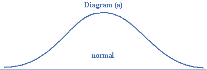
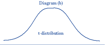
• An important property of the distribution of is that it is a normal distribution when the size of the sample is large. When the sample size is more than, we call it a large sample size. The shape of the population distribution does not
  matter. The population may be normal or non-normal, the distribution of  is normal for. But this is true when the number of samples is very large.
  As the distribution of random variable is normal,can be transformed into standard normal variable  where.

The distribution of has the t-distribution when the population is normal and . Diagram (a) shows the normal distribution and diagram (b) shows the t-distribution.

• The mean of the distribution of  is equal to the mean of the population. Thus  (Population mean). This relation is true for small as well as large sample size in sampling without replacement and with replacement.
• The standard error (standard deviation) of  is related with the standard deviation of population  through the relations:
  S.E.
  This is true when population is infinite which means  is very large or the sampling is done with replacement from finite or infinite population.

          S.E.
          This is true when sampling is without replacement from finite population. The above two equations between  and  are true both for small as well as large sample sizes.