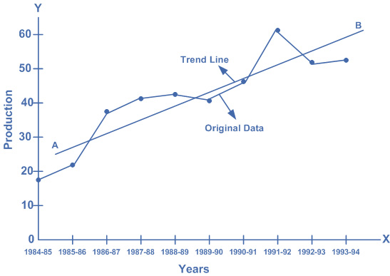
Method of Semi-Averages

This method is as simple and relatively objective as the free hand method. The data is divided in two equal halves and the arithmetic mean of the two sets of values of $$Y$$ is plotted against the center of the relative time span. If the number of observations is even the division into halves will be straightforward; however, if the number of observations is odd, then the middle most item, i.e.,$$\left( {\frac{{n + 1}}{2}} \right)th$$, is dropped. The two points so obtained are joined through a straight line which shows the trend. The trend values of $$Y$$, i.e., $$\widehat Y$$, can then be read from the graph corresponding to each time period.

Since the arithmetic mean is greatly affected by extreme values, it is subjected to misleading values, and hence the trend obtained by plotting by means might be distorted. However, if extreme values are not apparent, this method may be successfully employed. To understand the estimation of trends, using the above noted two methods, consider the following working example.

 

Example:

Measure the trend by the method of semi-averages by using the table given below. Also write the equation of the trend line with origin at 1984-85.

           

Solution:

Years	Values	Semi-Totals	Semi-Average	Trend Values
1984 – 85	18.6			28.664 – 3.656  = 25.008
1985 – 86	22.6			32.32 – 3.656 = 28.664
1986 – 87	38.1	161.6	32.32	32.32
1987 – 88	40.9			32.32 + 3.656 = 35.976
1988 – 89	41.4			35.976 + 3.656 = 39.632
1989 – 90	40.1			39.632 + 3.656 = 43.288
1990 – 91	46.6			43.288 + 3.656 = 46.944
1991 – 92	60.7	253.0	5.60	50.60
1992 – 93	57.2			50.60 + 3.656 = 54.256
1993 – 94	53.4			54.256 + 3.656 = 57.912

 

Trend for 1991 – 92 = 50.60
Trend for 1986 – 87 = 32.32
Increase in trend in 5 years = 18.28
Increase in trend in 1 year = 3.656

The trend for one year is 3.656. This is called the slope of the trend line and is denoted by b. Thus, b = 3.656. The trend for 1987 – 88 is calculated by adding 3.656 to 32.32 and similar calculations are done for the subsequent years. The trend for 1985 – 86 is less than the trend for 1986 – 87. Thus the trend for 1985 – 86 is 32.32 – 3.656 = 28.664. The trend for the year 1984 – 85 = 25.008. This is called the intercept because 1984 – 85 is the origin. The intercept is the value of $$Y$$ when X = 0.

The intercept is denoted by a. The equation of the trend line is $$\widehat Y = a + bX = 25.008 + 3.656X$$ (1984 – 85 = 0) where $$\widehat Y$$ shows the trend values. This equation can be used to calculate the trend values of the time series. It can also be used for forecasting the future values of the variable.